


By Masao Matsuda, PhD, CAIA, FRM, President and CEO of Crossgates Investment and Risk Management.
Equity volatility has a much more significant and multi-dimensional impact on portfolio construction and asset allocation than typically ascribed in investment literature or practiced in investment management. In this article, I will attempt to demonstrate how profoundly and widely equity volatility affects the returns and volatility of various asset classes and the correlations among these asset classes. Equity volatility is known to be more predictable than returns and correlations; hence, equity volatility is also arguably the most important determinant in pursuing successful portfolio construction and asset allocation.
A substantial portion of this article is derived from presentation materials that were used at the event jointly organized by the Chartered Alternative Investment Association’s (CAIA)’s New York Chapter and the Global Association of Risk Professionals’ (GARP’s) New York Chapter on July 19, 2023. Most data have been updated to include the returns of various indices and funds through September of 2023. Although the multi-dimensionality of equity volatility is also critical to alternative investment strategies, this article will focus on traditional assets for simplification.[i]
Equity volatility’s impact on returns of US equity and government bonds
Let us start by examining a long history of returns on US securities. Below is a performance example of US equity[ii] and government bonds[iii] classified by two equally-sized equity volatility regimes (high volatility and low volatility) over the 70-year period from 1949 to 2018. The volatility regimes are determined by ranking the standard deviation of daily returns for each month; those 420 months belonging to the top 50% are considered to be in the high volatility regime (hereinafter HVR), and the rest are considered to be in the low volatility regime (hereinafter LVR). These US securities’ returns and risk metrics are summarized below.
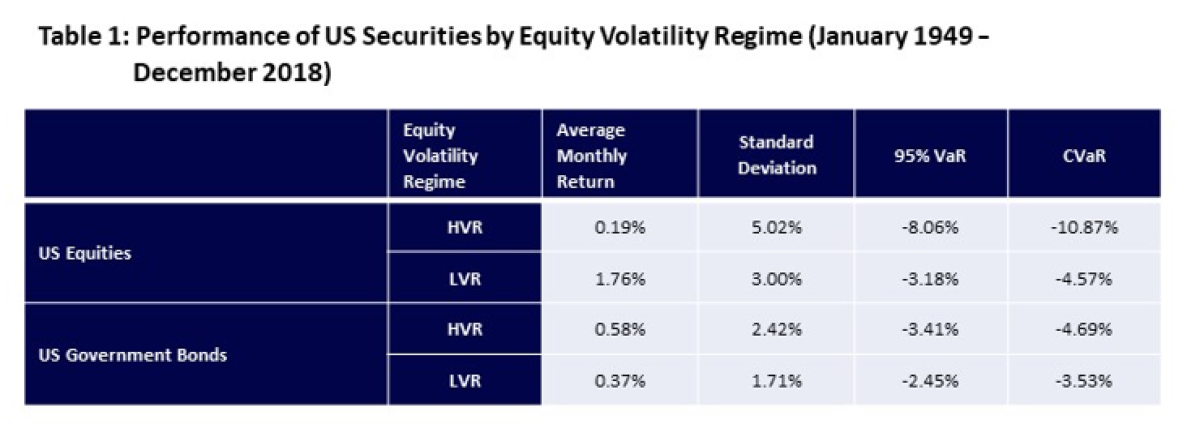
As shown in Table 1, the average return on investments in US equities in the LVR was 9 times higher (1.76% vs. 0.19%) than that in the HVR, though the risk (standard deviation) was naturally higher in the HVR (around 1.7 times higher risk). It is revealing that for half of the months in the 70-year period, those months in the HVR, US equity presumably generated returns that were less than a risk-free rate on average; in fact, the monthly average rate of return on three-month T-bills from January 1954 through December 2018[i] was 0.35%, much higher than 0.19%.
In terms of risk metrics, downside risk as measured by a 95% Value-at-Risk (VaR) indicates that in those 420 months in which equity volatility was low, in the LVR, 95% of the returns were higher than -3.18%. In addition, a Conditional VaR (CVaR), which is often viewed as a good measure of tail risk, shows that the 5% of the left tail distribution in the LVR had an average value of -4.57%.[ii] Compare these values to a -8.06% VaR and a -10.87% CVaR in the HVR. Thus, investing in US equity in the HVR came with a multitude of risks that were greater than in the LVR with a below risk-free rate of return.
By contrast, the average return on investments in US government bonds when equity’s volatility was high, in the HVR, was 1.6 times[iii] higher (0.58% vs. 0.37%) than in equity’s LVR, while the volatility was also higher in the HVR (1.4 times higher) than in the LVR. This also means that in the HVR months for US equities, government bonds delivered returns three times higher (0.58% vs. 0.19%) than those of US equity. It is hard to argue that equity volatility does not seriously affect bond returns. [Note to reader: in this article, whenever a reference is made to a volatility regime, it refers to US equity’s volatility even when discussing non-equity asset, like bonds, and investment strategies.]
Volatility Suprises
Further examining the relationships between equity volatility and returns, one realizes that changes or surprises in a volatility regime also affect returns very significantly. It is well known that volatility persists; when equity volatility is high, it is likely to remain high in the near future, and conversely, when the volatility is low, it is likely to remain low for the time being. Therefore, it is not unreasonable to assume that this month’s volatility regime remains the same next month, and if a change occurs, it can be viewed as a surprise.
In Chart 1 below, the “contemporaneous relationship” in the second row indicates the relationship between the current month’s volatility and return. The size of each bar is adjusted for frequency, though in this particular case both volatility regimes have 420 months each. The average monthly return before frequency adjustment for each regime is the same as shown in Table 1; in the chart one can visualize the fact that the average return for the LVR was 9 times higher than those of the HVR. In the rest of this paper, when expressions HVR and LVR are used, they refer to the “contemporaneous relationships” between volatility and returns.
The “naïve forecasts” in the first row assume that next month’s volatility regime remains the same as this month’s volatility regime. Interestingly, the frequency-adjusted returns between the two regimes appear to be roughly equal if one relies on the naive forecasts. What would account for the large difference in return attribution? By construction, the difference derives from the behaviors of the markets when the volatility regime changes, or volatility surprises occur, from High to Low or Low to High.
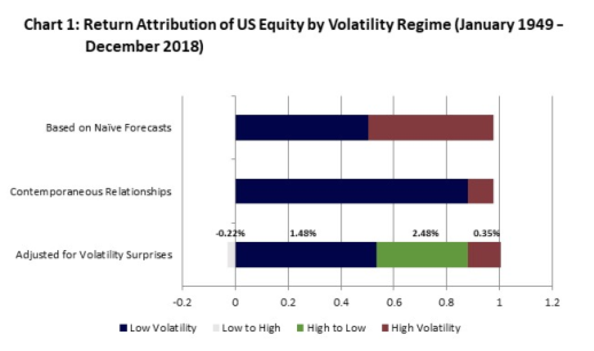
The third row in the chart considers the effects of the changes/surprises from one volatility regime to another. The size of each bar corresponds to return contributions after adjusting for frequencies. The numbers above each bar in the third row indicate an average of monthly returns before taking into account the frequency of each volatility regime or regime change. As one can see, the largest contributions were made in those months with consistently Low Volatility (an average return of 1.48% for 303 months) and those months when the changes occurred from High Volatility to Low Volatility (an average return of 2.48% for 117 months). Consistently high volatility months also contributed to positive returns (an average of 0.35% for 302 months). By contrast, when the volatility regime changes from Low to High, the returns were negative (an average return of -0.22% for 118 months).
The point of the above exercise was not to demonstrate the reasonable accuracy of the naïve forecasts, though the naïvely forecast volatility regime was consistent with the actual volatility regime around 72% of the months (302 out of 420 months for the HVR and 303 out of 420 months for the LVR). It was rather to highlight the importance of the role that volatility changes or surprises play in equity returns. In addition, US equity’s volatility surprises affect other asset classes significantly, including non-equity asset classes, which will be discussed in the next section.
Equity volatility’s impact on returns of other assets
Before delving into the effects of US equity’s volatility on other equity and non-equity asset classes, let us examine the relationship between the S&P 500 index[i] and its volatility. This time we will focus on the more recent 19-year period. It will serve as a base for comparison with other asset classes, many of which lack return data going back in history for 70 years.
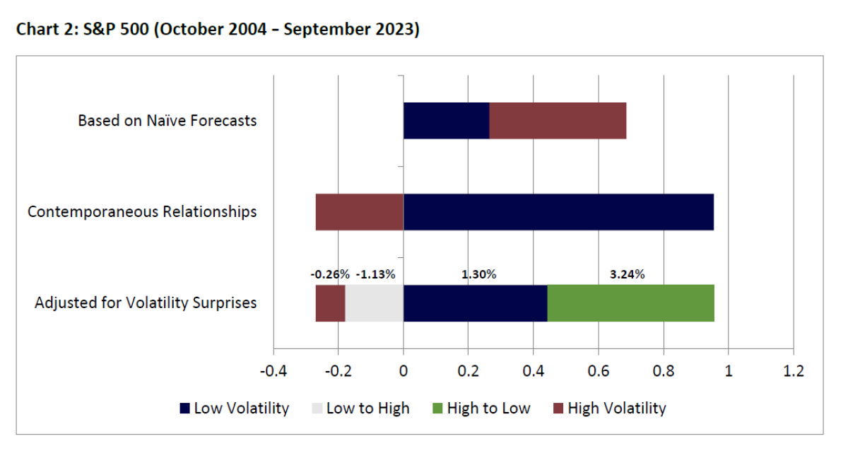
Chart 2 shows that in terms of the contemporaneous relationship during the recent 19-year period (October 2004 to September 2023), the S&P 500 contributed returns of nearly 1% per month after adjusting for frequency in the Low Volatility months. On the other hand, the S&P 500 lost nearly 0.3% per month in the High Volatility months. This is in stark contrast to a relatively large contribution in the High Volatility months based on the naïve forecasts. By examining the 3rd row, one realizes that the differences are due to the volatility surprises of moving from High to Low, as well as to the surprises going from Low to High. In terms of absolute numbers, in those months in which the volatility regime shifted from High to Low, returns of 3.25% per month were added, whereas as in those months in which the regime shifted from Low to High, losses of 1.13% per month on average were experienced. In 36 out of 114 months, the volatility regime changed from High to Low. Similarly, in 36 out of 114 months, the volatility regime changed from Low to High.
Though not shown to avoid repetitive charts, a very similar pattern was observed for the S&P Small Cap index, as well as the MSCI EAFE index during the same period. In addition, the S&P Mid-Cap Index (not shown) and the MSCI Emerging Market Equity Index (see Chart 3) also exhibited similar patterns. However, in the High Volatility months without volatility surprises, the equity securities in these two indices made a small positive contribution to returns.[i]
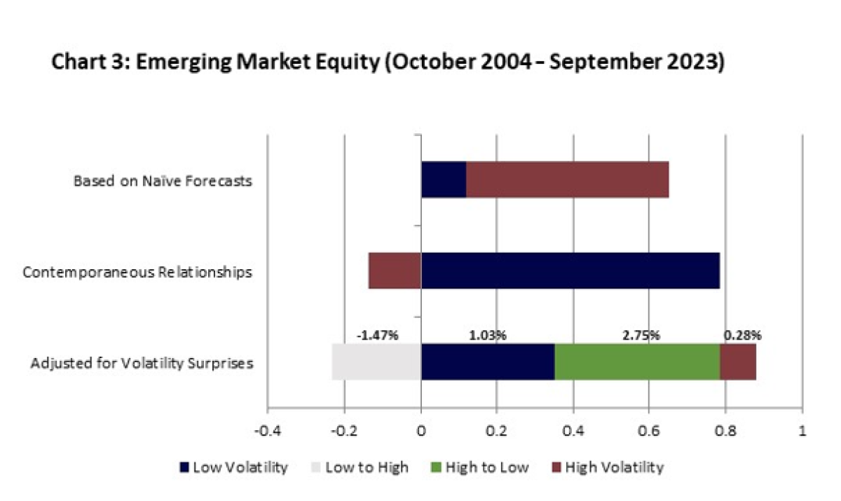
Chart 4 shows the breakdown of the returns of a REIT (VNQ)[i] during the same period. A major difference from the previous charts is that under any volatility scenarios the REIT made at least a small contribution. As in the case of the S&P 500 and other equity indices, the REIT made the largest contribution to returns in those months in which the volatility regime changed from High to Low with an average monthly return of 2.24%, followed by the steadily Low Volatility months with an average monthly return of 0.84%.
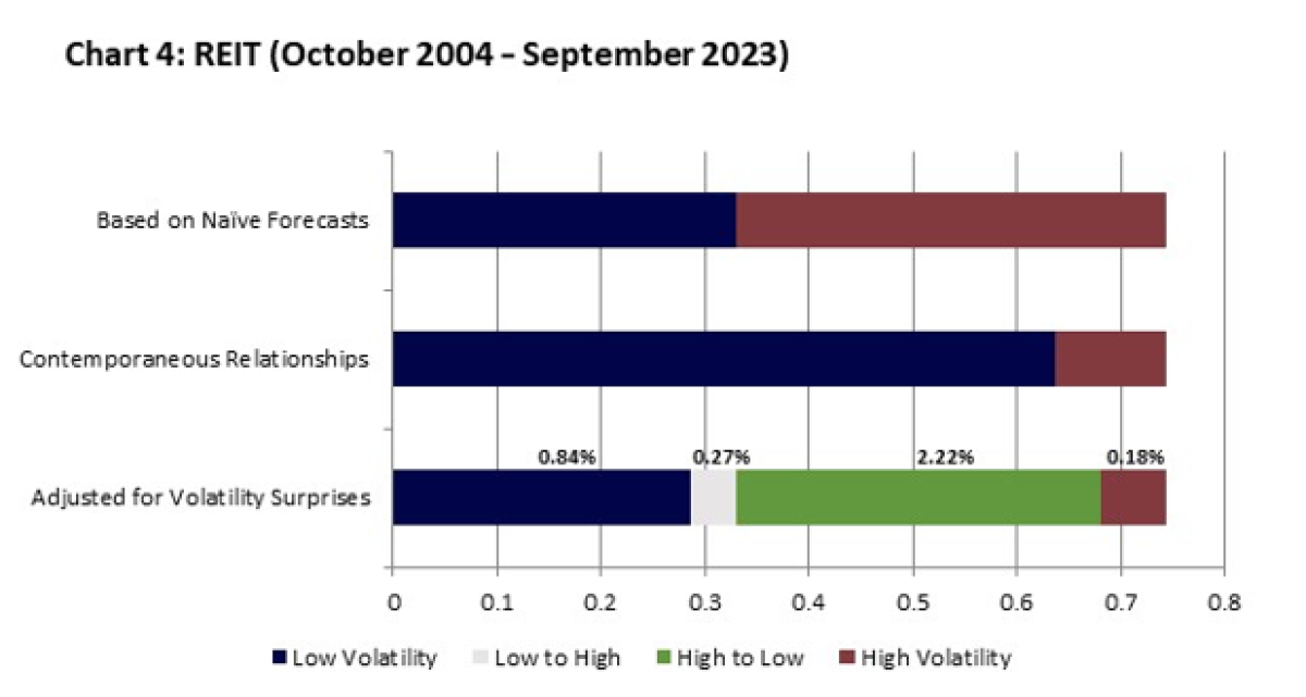
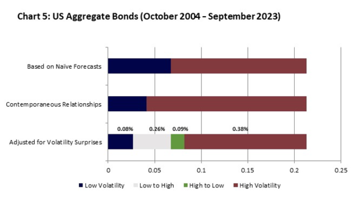
Chart 5 represents a good example of how fixed-income securities tend to behave in relationship to equity volatility. In both contemporaneous relationships and based on naïve forecasts, in the High Volatility regime, US aggregate bonds (AGG)[i] performed much better than in the Low Volatility regime. Moreover, when adjusted for volatility surprises, one can readily see that the Low to High changes contributed more than the High to Low changes. These facts clearly point to the potential diversification benefits of bonds to an equity-oriented portfolio, which tends to suffer in the HVR and the changes from Low to High volatility. However, in terms of an absolute level of returns, AGG generated only 0.21% a month on average.
A similar pattern is observed for US TIPS[i] (not shown). While the returns were slightly better than AGG with an average 0.27% per month, most return contributions also occurred in the High Volatility months with an average monthly return of 0.51%. One difference from AGG is that the High to Low changes made a relatively large contribution with an average return of 0.29% per month.
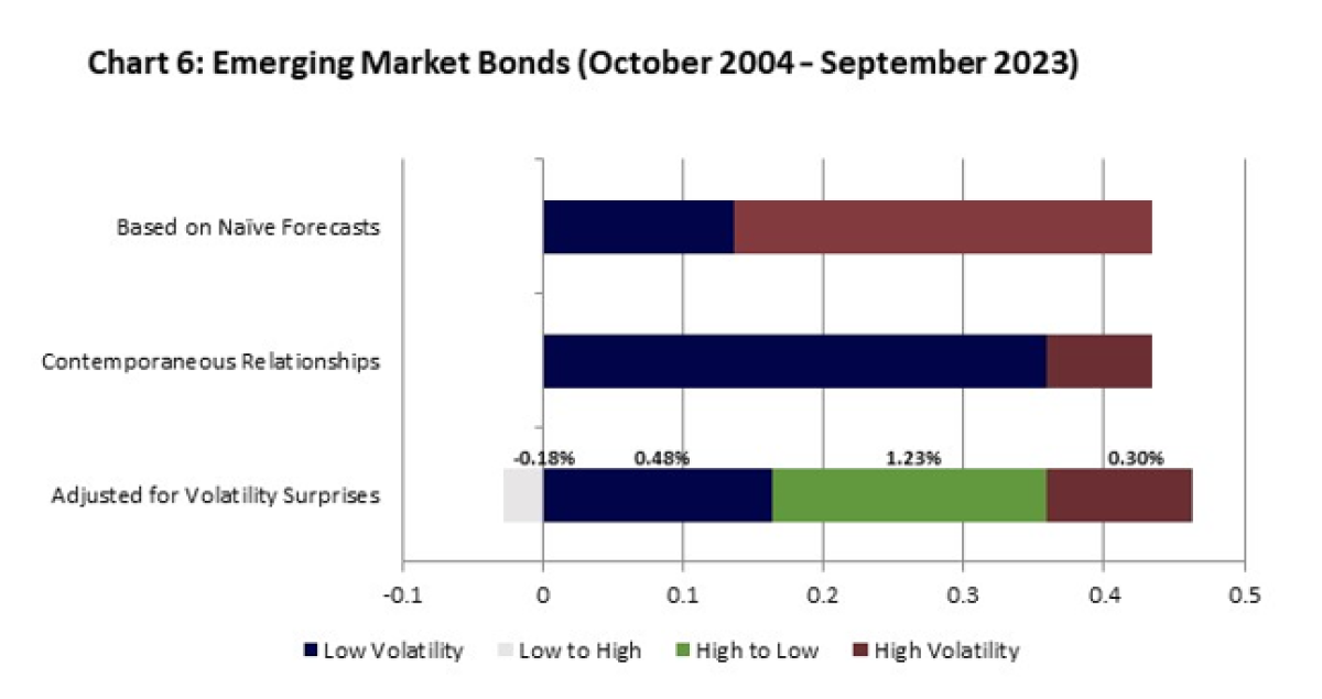
Chart 6 shows the behaviors of emerging market bonds[ii] (PREMX). Interestingly, in terms of contemporaneous relationships, these bonds made most return contributions in the LVR, similar to equities and REIT. A closer examination reveals that the High to Low changes and the LVR made roughly equal frequency-adjusted contributions (0.19% and 0.16% respectively). In addition, like US equity, the Low to High changes resulted in negative returns.
Unlike emerging market bonds, the returns of international bonds[i] (PFORX, not shown) exhibited a pattern similar to those of AGG or TIPS. While representing the performance of non-US developed countries’ bonds, these returns were higher than AGG or TIPS with a 0.39% average monthly return. The largest contribution of 0.21% was made in the steadily High Volatility months, followed by the contribution of 0.14% in the steadily Low Volatility months. The volatility changes in either direction made a positive but small contribution each.
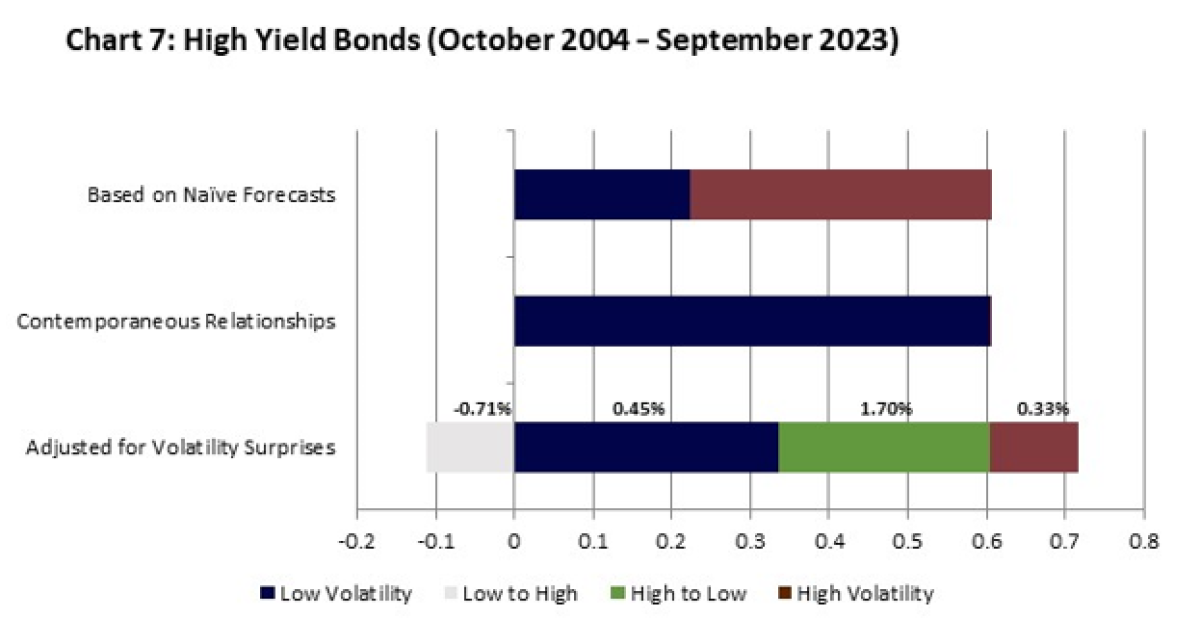
High yield bonds[i] are known to behave like equity securities. Not surprisingly, Chart 7 indicates that nearly all return contributions were made in the LVR in terms of contemporaneous relationships (in the HVR these bonds made a miniscule contribution of 0.001% to returns). When adjusted for frequency, these bonds also made a relatively large contribution in the High to Low volatility changes with an average monthly return of 1.70%. The difference from equities lies in the fact that in the High Volatility months these bonds also made positive contributions after adjusting for frequency in the recent 19-year period.
Correlations and volatilities under different equity volatility regimes
If the volatility of US equity affects the returns of various asset classes, correlations among these asset classes and the volatilities of each asset class are ipso facto affected as the returns are the sole inputs to calculate these parameters. It follows that one should expect a different correlation structure between the HVR and LVR.
One of the fundamental tenets in modern portfolio theory is that correlations play the most critical role in diversifying investment risks. In general, the lower the correlation among securities or asset classes the higher the diversification effects, and vice versa. Table 2 shows two sets of numbers for each combination of nine asset classes. The top row in each cell indicates the difference in correlation between HVR and LVR. When HVR’s correlation is higher, it results in a positive number. When HVR’s correlation is lower, it results in a negative number and is indicated in red in the table. The second row in each cell is the correlation coefficient between each pair of assets throughout the period without regard to volatility regimes.
It is astounding that for most combinations of asset classes the HVR had higher correlations than in the LVR, and in many cases the difference in correlations between the two volatility regimes was nearly 0.3 or higher. The only four exceptions are those involving REIT, TIPS or US aggregate bond (Agg). Even among those cases, however, the maximum difference was -0.08, indicating that the LVR did not deliver meaningfully greater diversification benefits than the HVR. Clearly, however, the LVR has a potential to deliver better diversification benefits. Needless to say, when a correlation structure differs, an asset allocation policy should be pursued accordingly.
Market participants and investment professionals often lament that diversification benefits disappear when they are needed most. In fact, as demonstrated in Table 2, when equity volatility goes up, the correlations among asset classes go up and the benefits of diversification are substantially diminished. This is another reason why one should explicitly consider the multidimensional impact of equity volatility in constructing a portfolio or performing asset allocation.
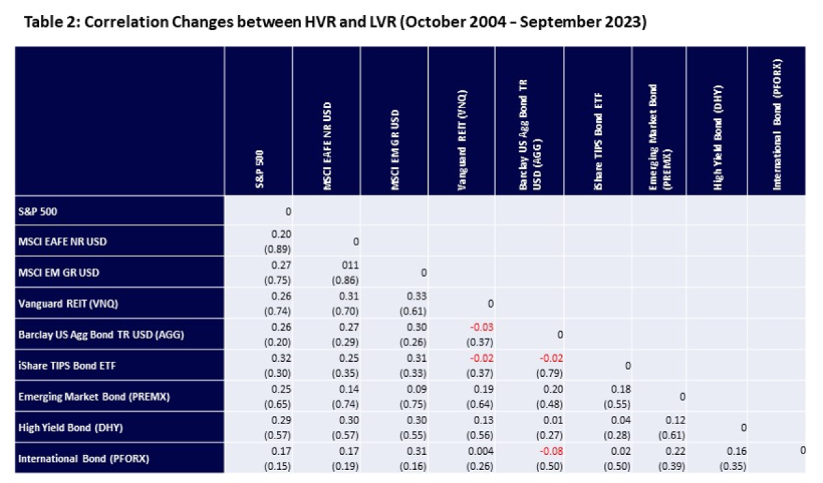
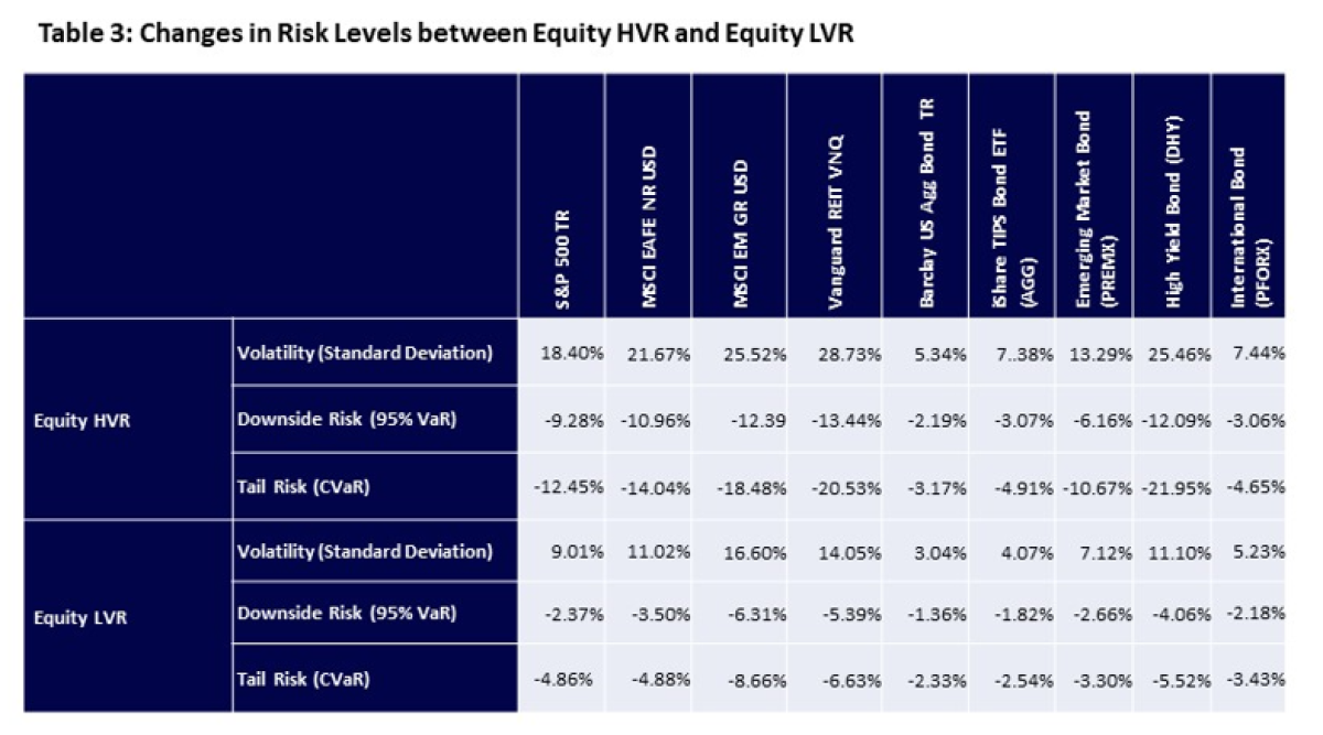
Table 3 compares the changes in three risk metrics between Equity’s HVR and LVR. It is apparent that regardless of asset classes, equity volatility had a significant impact on volatility, downside risk and tail risk of each asset class. In all cases, the levels of risk were higher in the HVR. In particular, equity and equity-type assets tended to show roughly twice as high a volatility in the HVR compared to that in the LVR. Moreover, also in all cases, both downside risk and tail risk were much smaller in the LVR. Just as in the correlations among asset classes, equity volatility has an unmistakable impact on the risks of other assets.
For both portfolio construction and asset allocation, the main inputs are (1) expected returns of assets, (2) the volatilities of these assets, and (3) the correlations among these assets. As has been demonstrated, depending on S&P 500’s volatility regime, these inputs exhibit different tendencies. Therefore, the role of equity volatility goes beyond being a single input in the portfolio construction and asset allocation processes; it directly impacts all three types of inputs, confirming multi-dimensionality of volatility,
In addition, the predictability of volatility is known to be higher than that of expected returns or correlations. As a matter of fact, as discussed earlier, volatility surprises occurred in 28% of the months when based-on native forecasts. In other words, in 72% of the months the volatility regime remained unchanged.
Conceivably, due to the one-dimensional way in which investment professionals are trained to treat the main inputs into an asset allocation process, they may not properly focus on the muti-dimensionality of volatility’s impact. Bearing in mind the empirical evidence demonstrated above, one should not maintain a singular allocation strategy without regard to the equity volatility regime. In particular, the HVR calls for a special consideration since, in all nine asset classes, the risk metrics tend to be higher with lower returns. Furthermore, in the HVR most of these asset classes provide smaller diversification benefits. In the next section, an example of an overlay strategy that will be engaged only when high volatility months are expected will be demonstrated.
Use of risk premia factors for asset allocation
Suppose that one can predict next month’s equity volatility to a reasonable degree and that one has identified five risk premia factors that tend to provide modest returns with relatively low risks in the high volatility regime. Suppose also that the performance of these factors does not deteriorate significantly even in the presence of volatility surprises, and that they have low-to-negative correlations among each other. If factors are chosen to represent risk premia from different asset classes/strategies, one could implement factor-based asset allocation. For simplicity, let us call such a portfolio “Dynamic Factor Portfolio” or “DFP” for short.
While there are many ways to implement such a strategy, an example given in Table 4 assumes that 90% of the assets are invested in the S&P 500 index, and the rest are utilized as a margin for overlay of the DFP when an HVR is predicted.[i] Crossgates Investment and Risk Management’s proprietary algorithm was utilized to make predictions of equity volatility.
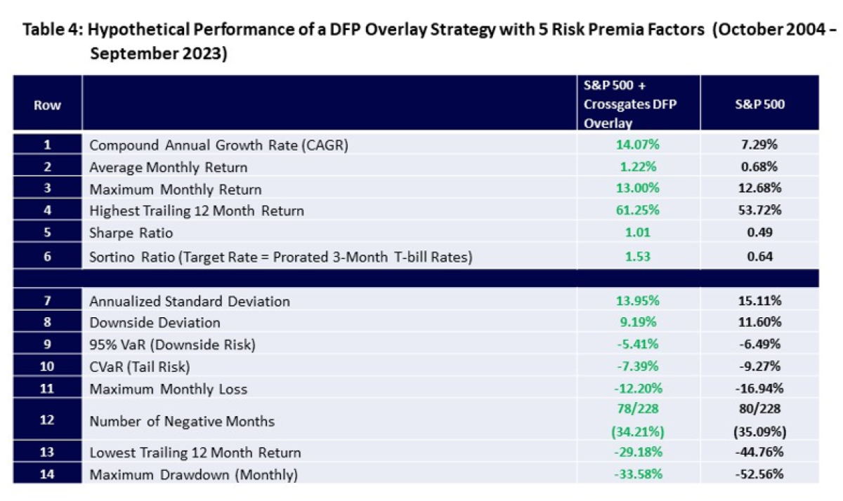
In Table 4, results of Crossgates’ DFP Overlay strategy with five risk premia factors[ii], as applied to the S&P 500, are shown. The period for this historical simulation is from October 2004 to September 2023, and during the subject period, when an HVR is predicted the combination of the five risk premia factors are engaged.[iii] The notional amount for each factor is adjusted so that each factor’s volatility is the same as that of the S&P 500 for the same period, i.e., 15% per annum. To the extent that these factors are uncorrelated, or inversely correlated, to each other, however, the overall volatility of the factor portfolio becomes about a half of S&P 500’s 15%.
The numbers in green in the table indicate higher returns/ratios in row 1 through row 6, and lower risks in row 7 through row 14 between (1) the S&P 500 with Crossgates DFP Overlay and (2) the S&P 500. The returns are net of estimated transaction costs for swap contracts which deliver the performance of the risk premia factors (an average transaction cost of 0.114% per month for the relevant period).
As one can see, in all return metrics and risk metrics, (1) the S&P 500 with Crossgates DFP Overlay dominates (2) the S&P 500. For instance, the compound annual growth rate (CAGR) became twice as high after applying the DFP Overlay to the S&P 500. A Sharpe radio was twice as high and a Sortino ratio was more than twice as high. In other return measures the application of the overlay also resulted in better performances. In the meantime, all the risk metrics became lower after applying the overlay. In particular, the lowest trailing 12-month return (-29.18% vs -44.76%), as well as, the maximum drawdown (-33.58% vs. -52.56%) showed a substantial improvement.
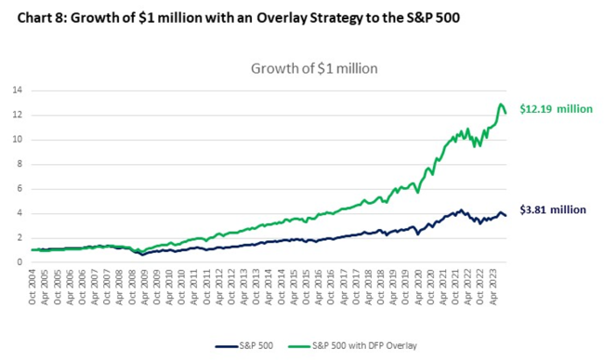
Chart 8 shows the growth of $1 million invested for the period October 1, 2004 to September 30, 2023. As demonstrated in Table 4 above, applying the Crossgates DFP Overlay results in the generation of returns significantly higher, roughly twice as high per year, compared to those of the S&P 500. When the DFP Overlay is applied, the compounded annual growth rate of 14.07% contrasts markedly with the much lower growth rate of 7.29% for the S&P 500 on its own. In fact, the final investment becomes nearly 4 times as large ($12.19 million vs. $3.81 million). Importantly, as was shown in Table 4, this was accomplished with smaller risk (volatility: 13.95% vs 15.11%), smaller downside risk (95% VaR: -5.41% vs. -6.549%), as well as, smaller tail risk (CVaR: -7.39% vs. -9.27%). Hence, the benefits of applying the DFP Overlay are indisputable.
Conclusion
A multi-dimensional impact of US equity volatility has been discussed in this article. By dividing samples of return data into two groups (equity’s high volatility regime or HVR and low volatility regime or LVR), one could readily see how the volatility of US equity affected other asset classes’ returns, various types of risks (volatility, downside risk, and tail risk) of the asset classes, as well as, the correlations among these asset classes. In retrospect, it was apparent that US equity’s volatility affected these parameters as they were calculated using only return numbers, and they were clearly affected by such volatility. The examination of equity volatility regimes also revealed why under certain conditions the diversification benefits become less attainable.
In order to demonstrate the importance of taking into account equity volatility in a multitude of ways in asset allocation, the results of an historical simulation were presented. No optimization was involved in the simulation; it showed that by merely utilizing five risk premia factors as an overlay when an HVR was predicted, one could enhance returns while lowering the risks of the underlying strategy. This result points out that proactively responding to different volatility regimes may be the best diversifier of the various risks in implementing asset allocation and portfolio construction. It is also critical to make such an implementation robust enough for volatility surprises.
In this article, only two regimes were discussed, highlighting the significance of equity volatility and its changes. For practical application, however, one can assume a higher number of volatility regimes for the purpose of better representing the relationships between volatility and returns. Moreover, the number of months in each regime need not be made equal. Afterall, one does not know how many months will fall in the category of high volatility ahead of time. The simulation results shown in Table 4 indeed reflect such an endeavor at Crossgates Investment and Risk Management, and the DFP Overlay can be applied to many asset classes, as well as to investment strategies that tend to suffer in equity’s high volatility regime.
[1] Most hedge fund strategies tend to show a similar tendency, which will be discussed in the article. This happens due to the fact that these hedge fund strategies have relatively high beta exposure to equity risk. See, for instance, https://caia.org/blog/2020/05/19/time-varying-equity-volatility-markedl….
[1] Data Source: Kenneth R. French Data Library, Tuck School of Business at Dartmouth. It covers equity securities in NYSE, AMEX, and NASDAQ
[1] Data source: International Government Bond Returns Since 1947, figshare. Dataset.
[1] The data prior to January 1954 was not available.
[1] Among risk professionals, it is common to cite only the absolute numbers for VaR and CVaR. For more intuitive understanding, however, a minus sign is attached in this article when expressing these risk measures.
[1] 0.584%/0.366%=1.596.
[1] The monthly returns of the S&P 500 index that are adjusted for split and dividends. Data source: Yahoo Finance. In the rest of the article, the same data for the S&P 500 was utilized.
[1] For the S&P Mid-Cap Index, the steadily High Volatility months contributed 0.005% during the relevant period.
[1] Vanguard REIT, VNQ.
[1] Barclay US Aggregate Bond Total Return. Most funds were chosen for the analyses primarily based on the availability of data going back to the October 2004.
[1] iShares TIPS Bond ETF by BlackRock.
[1] Emerging market bond fund by T. Rowe Price.
[1] Vanguard international bond ETF, PFORX.
[1] Credit Suisse high yield bond fund, DHY.
[1] When a high volatility month is not predicted, the 10% of assets earn the 3-month T-bill rates.
[1] These factors are implemented through swap contracts offered by investment banks.
[1] The factors were chosen based on a longer data, using criteria that eliminate factors with high downside and tail risks. The most recent years reflect an out-sample performance.
[i] When a high volatility month is not predicted, the 10% of assets earn the 3-month T-bill rates.
[ii] These factors are implemented through swap contracts offered by investment banks.
[iii] The factors were chosen based on a longer data, using criteria that eliminate factors with high downside and tail risks. The most recent years reflect an out-sample performance.
[i] Credit Suisse high yield bond fund, DHY.
[i] Vanguard international bond ETF, PFORX.
[i] iShares TIPS Bond ETF by BlackRock.
[ii] Emerging market bond fund by T. Rowe Price.
[i] Barclay US Aggregate Bond Total Return. Most funds were chosen for the analyses primarily based on the availability of data going back to the October 2004.
[i] Vanguard REIT, VNQ.
[i] For the S&P Mid-Cap Index, the steadily High Volatility months contributed 0.005% during the relevant period.
[i] The monthly returns of the S&P 500 index that are adjusted for split and dividends. Data source: Yahoo Finance. In the rest of the article, the same data for the S&P 500 was utilized.
[i] The data prior to January 1954 was not available.
[ii] Among risk professionals, it is common to cite only the absolute numbers for VaR and CVaR. For more intuitive understanding, however, a minus sign is attached in this article when expressing these risk measures.
[iii] 0.584%/0.366%=1.596.
[i] Most hedge fund strategies tend to show a similar tendency, which will be discussed in the article. This happens due to the fact that these hedge fund strategies have relatively high beta exposure to equity risk. See, for instance, https://caia.org/blog/2020/05/19/time-varying-equity-volatility-markedl….
[ii] Data Source: Kenneth R. French Data Library, Tuck School of Business at Dartmouth. It covers equity securities in NYSE, AMEX, and NASDAQ
[iii] Data source: International Government Bond Returns Since 1947, figshare. Dataset.
About the Author:
Masao Matsuda, PhD, CAIA, FRM is President and CEO of Crossgates Investment and Risk Management. He has over three decades of experience in the global financial services industry. He has acted as CEO of a US broker-dealer and CEO/CIO of a number of investment management firms. In addition to his broad knowledge of alternative investments and traditional investments, he also possesses a technical expertise in financial modeling and risk management. He is experienced as a corporate director for operating and holding companies, and as a fund director for offshore investment vehicles.

Prior to founding Crossgates Investment and Risk Management, Masao spent 18 years with the Nikko group of companies of Japan. For the last seven years of his career at Nikko, he served as President/CEO of various Nikko entities in the US, and as a director of Nikko Securities Global Holdings. He received his Ph.D. in International Relations from Claremont Graduate University. He holds CAIA and FRM designation. He is a member of the Steering Committee of CAIA’s New York Chapter, as well as a committee member of GARP’s New York Chapter. He can be reached at matsuda@crossgates-im.com.